2024 · Physical Review D · Open access on arXiv
Decoding the B⁺ → K⁺ νν excess at Belle II: Kinematics, operators, and masses
Belle II has measured more B⁺ → K⁺ νν decays than the Standard Model predicts — about 2.7σ more, a tantalising but not yet decisive hint. This paper asks what the unseen “νν” could really be, fits the leading new-physics scenarios to the published event distribution, and finds that the data prefer a pair of invisible particles produced by a vector current with a mass around 0.6 GeV — a possible dark-matter particle — with a single invisible particle of about 2 GeV a close second.
Published in: Kåre Fridell, Mitrajyoti Ghosh, Takemichi Okui, Kohsaku Tobioka, Decoding the B → Kνν excess at Belle II: kinematics, operators, and masses, Phys. Rev. D 109 (2024) 115006. doi:10.1103/PhysRevD.109.115006 · free preprint on arXiv
Background: a rare decay with a surprise
The decay B⁺ → K⁺ νν is a rare process in the Standard Model (SM): a b quark turns into an s quark and the energy is carried away by a neutrino–antineutrino pair, which no detector can see. The rate is tiny — the SM predicts a branching fraction of (5.58 ± 0.37)×10−6 — but it is also one of the cleanest places to look for new physics, because the theory uncertainty is small.
In 2023 the Belle II experiment reported a measurement using a new inclusive tagging method: a branching fraction of (2.7 ± 0.5 (stat) ± 0.5 (syst))×10−5. Combining with the older hadronic-tagging analysis gives (2.3 ± 0.5 (stat) +0.5−0.4 (syst))×10−5 — about 2.7σ above the SM prediction. Not a discovery, but worth taking seriously.
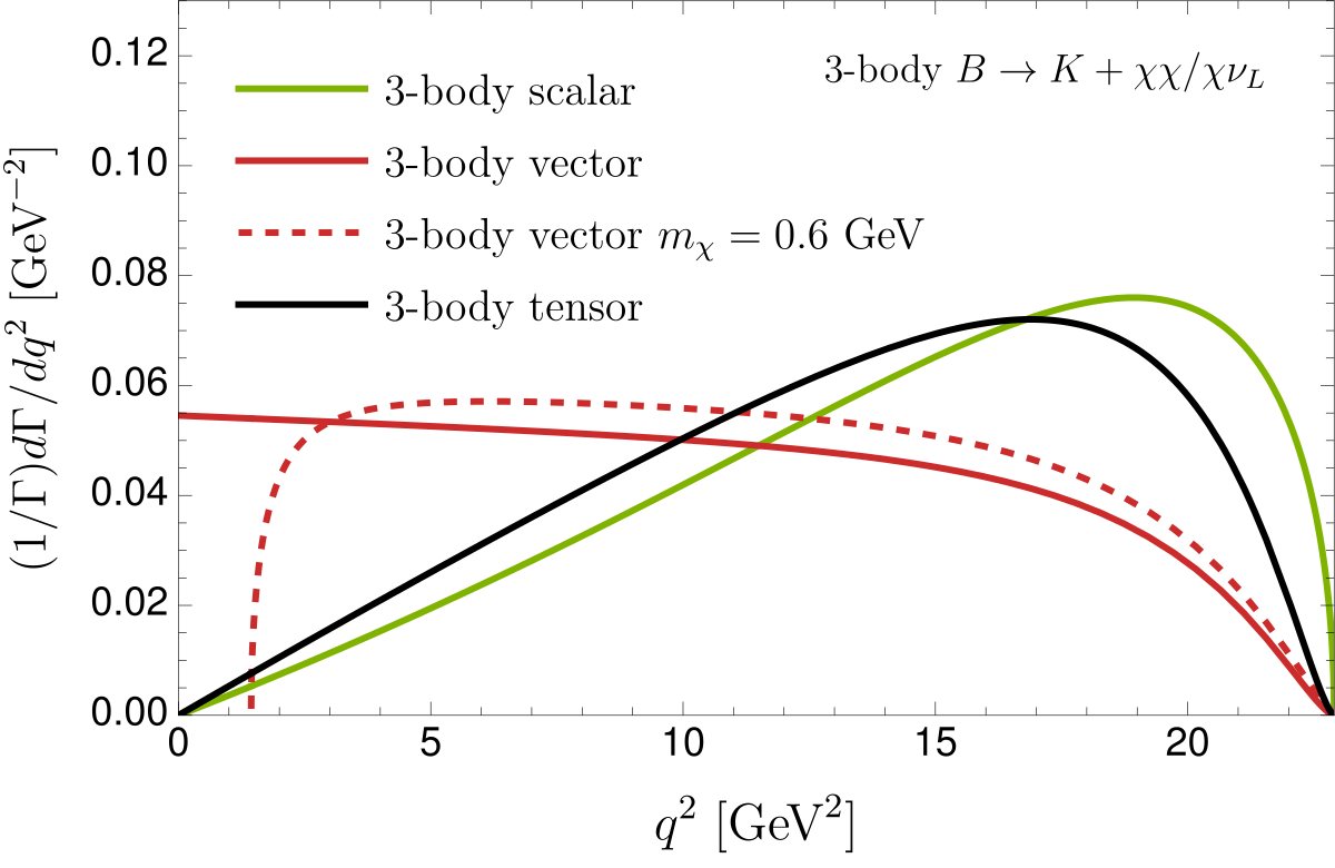
If the excess is real and new physics is responsible, the invisible “νν” does not have to be two ordinary neutrinos. It could be a single new invisible particle X (a “2-body” decay, B → K X), or a pair of new particles χχ (a “3-body” decay, B → K χχ). The pair could be produced through three different kinds of interaction — a scalar, a vector, or a tensor current — and each option predicts a different shape for how the events are distributed in the missing mass. That shape is the key to telling the scenarios apart.
What the paper does
The authors perform a careful statistical analysis of the published Belle II event distribution, then add older BaBar data as a cross-check:
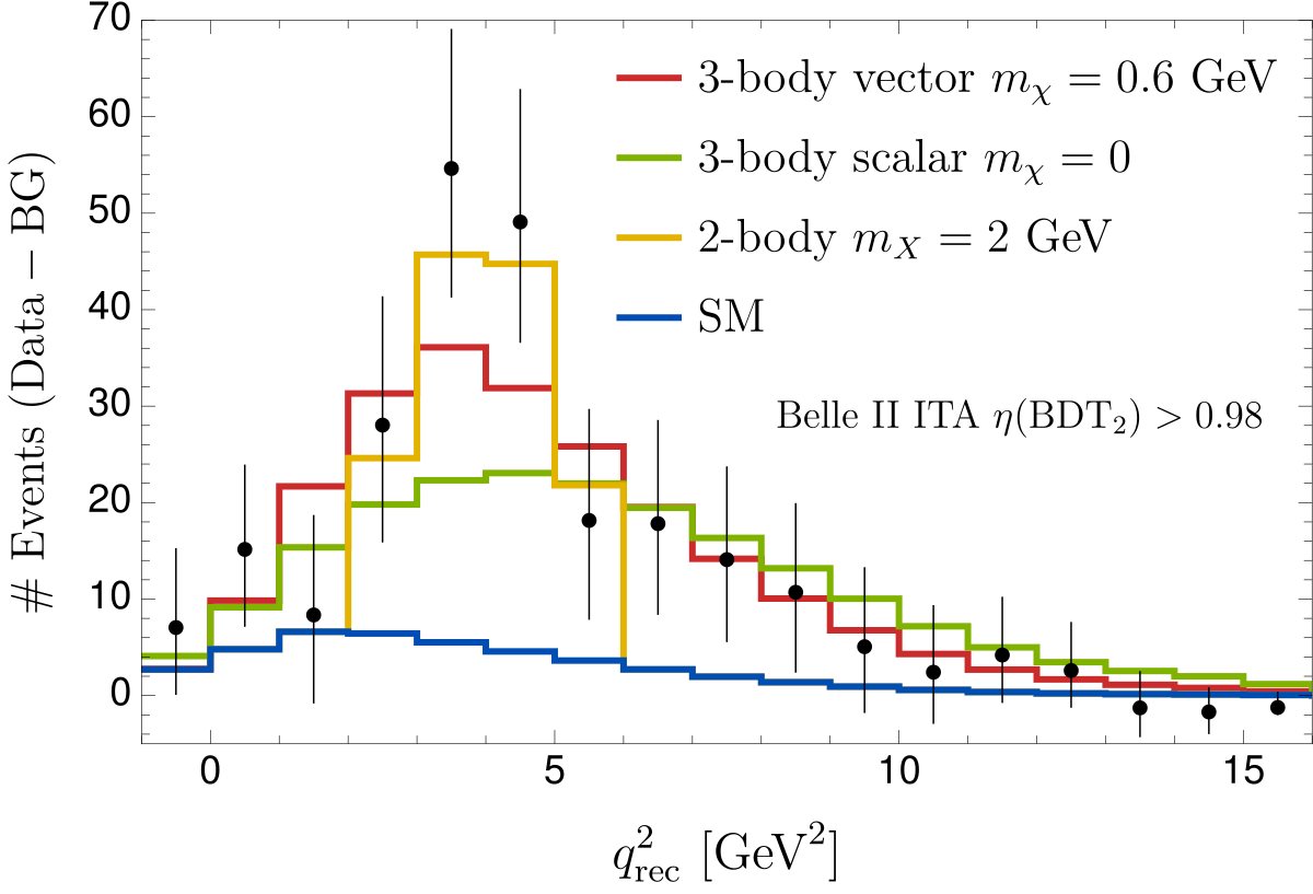
- Handles the tricky variable. Inclusive tagging does not reconstruct the tagged B meson, so Belle II bins events in q2rec, an approximation of the true momentum transfer q2 = (pB − pK)2. The paper simulates how each scenario's true q2 distribution gets smeared over q2rec (for example, a 2-body decay with mX = 2 GeV is spread over about 2.5 GeV2) before comparing with data.
- Recovers the signal efficiency. The efficiencies published by Belle II do not apply to the tight selection where the excess appears, so the authors tune a q2-dependent efficiency until their SM-like (vector-current) prediction reproduces the reported event shape.
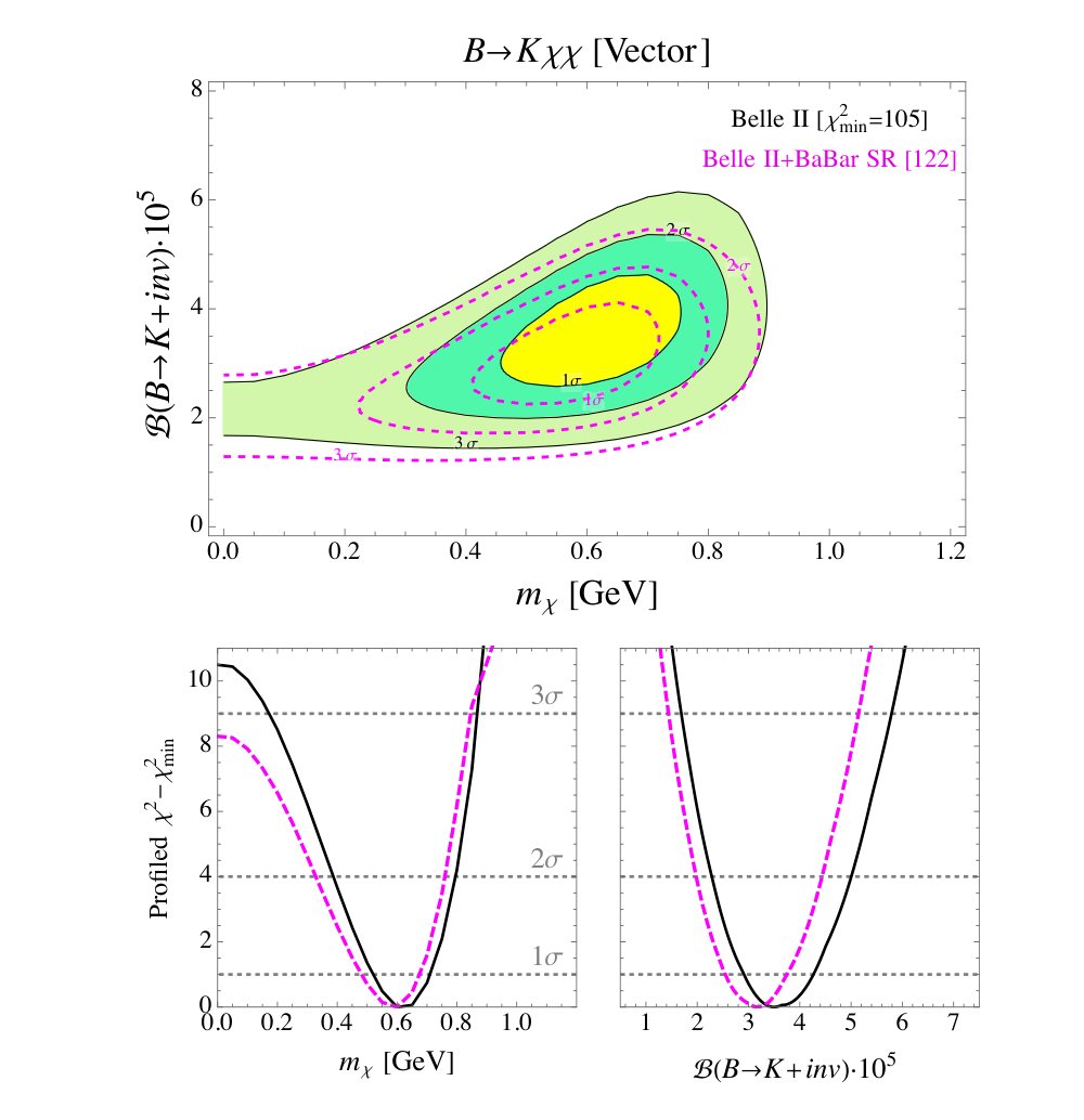
- Fits each scenario. Using a binned Poisson likelihood on the 3.99×10⁸ B mesons in the Belle II sample, they fit the branching fraction and the new-particle mass for the 2-body case and for 3-body scalar, vector, and tensor currents, scanning the mass including the massless limit and masses around 0.6 GeV. As a check, their fit reproduces Belle II's inclusive-tagging result: (2.6 ± 0.4 (stat))×10−5.
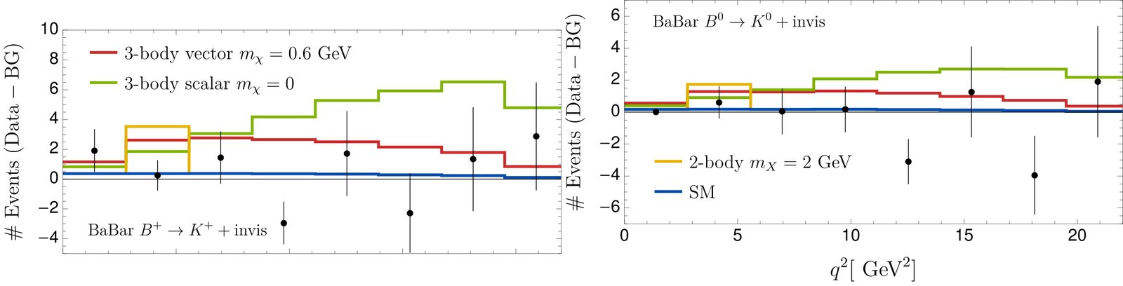
- Cross-checks with BaBar. The older BaBar measurements of B → Kνν (471×106 BḫB pairs) used the true q2 with good resolution, so they can discriminate between scenarios — especially at high q2, where Belle II has almost no efficiency.
- Translates results into new-physics scales. Each best fit is converted into a bound on the heavy energy scale (Λ) or coupling strength of the operator that would cause the decay.
For the 3-body scenarios the authors deliberately pick operators that have little effect on the related decay B → K*νν — in particular a pure vector current rather than the SM-like vector-minus-axial-vector — since Belle II has placed an upper limit on B → K*νν but has not yet measured it.
What they found
Best fit: vector current, mχ ≈ 0.6 GeV
The most favoured interpretation is B⁺ → K⁺χχ via a vector current, with mχ = 0.62 +0.10−0.09 GeV and branching fraction (3.5 +0.8−0.6)×10−5. If χ is stable, it is a dark-matter candidate.
Close second: 2-body, mX ≈ 2 GeV
A single invisible particle X with mX = 1.97 ± 0.05 GeV and branching fraction (0.79 +0.16−0.13)×10−5 fits almost as well as the vector scenario.
Scalar and tensor need much more rate
Their best fits require branching fractions a few times larger — (7.9 +1.6−1.5)×10−5 for the scalar (best at mχ = 0) and (6.4 ± 1.2)×10−5 for the tensor — because their event shapes peak where the detector is least efficient.
The SM fits worst
Of all the hypotheses tested, the Standard-Model shape is the worst fit to the Belle II data, while the SM-like massless vector case is also clearly disfavoured. Even if unaccounted systematic uncertainties halved the χ², those cases would remain disfavoured.
BaBar sharpens the picture
Adding the past BaBar data leaves the preferred parameters essentially unchanged, but increases the fit-quality gap between the 2-body scenario and the best 3-body scenario (from Δχ² ≈ 2 to ≈ 5) and severely worsens the scalar and tensor cases, which would have produced an excess at high q2 that BaBar did not see.
New-physics scales
The best fits correspond to a vector-current scale ΛV ≈ 6.5 TeV, a scalar-current scale ΛS ≈ 4.1 TeV, and an effective 2-body coupling λX ≈ 3×10⁻⁴.
| Dataset | 2-body | V (mχ = 0) | V′ (mχ ≈ 0.6 GeV) | Scalar | Tensor | SM |
|---|---|---|---|---|---|---|
| Belle II inclusive tagging | 6.8 | 15.2 | 4.7 | 15.1 | 11.9 | 44.6 |
| + BaBar signal region | 27.6 | 30.4 | 22.1 | 31.8 | 29.8 | 61.0 |
| + BaBar, including q2 ≳ 8.4 GeV2 | 73.3 | 78.8 | 72.9 | 90.2 | 86.9 | 106.7 |
In one line: If the Belle II excess is new physics, the shape of the data prefers a B⁺ → K⁺χχ decay through a vector current with χ around 0.6 GeV — a possible dark-matter particle — while a single invisible particle of about 2 GeV remains a close competitor, and scalar or tensor explanations need several times more events than the measurement allows at face value.
Why it matters
An excess that is only 2.7σ is exactly the situation where interpreting the data correctly matters most: new physics may be visible, or the measurement may fluctuate back to the Standard Model. This paper shows that the full shape of the event distribution — not just the total rate — already carries enough information to prefer some scenarios over others. It also delivers a cautionary lesson: if you ignore that Belle II reports a smeared variable and that the detector's efficiency varies with q2, you can misread what branching fraction the data actually demand (for the scalar current, by roughly a factor of three). Future Belle II data, with more events and better reconstruction, will either make the χ or X hypothesis testable or let the excess fade away; in the meantime, this analysis maps out precisely what to look for.
Key concepts
- Branching fraction
- The probability that a particle decays in a particular way. Here, the chance that a B⁺ meson turns into a K⁺ plus invisible particles; it is tiny, of order ten per million.
- Momentum transfer q2
- The squared mass of the invisible system in the decay, computed from the energies and momenta of the B and K mesons. Its distribution is a fingerprint of the underlying interaction — and of how heavy the invisible particles are.
- q2rec
- Belle II's approximation to q2: because the tagged B momentum is not fully reconstructed in inclusive tagging, events are binned in this reconstructed variable, which smears each true q2 over a range of values.
- Scalar, vector and tensor currents
- Three ways the b quark can transform into an s quark while emitting the invisible pair, combining the quark spins and momenta differently — a scalar, a vector or a tensor interaction. Each predicts a different q2 shape.
- Profile likelihood
- A statistical tool for focusing on one parameter at a time: for each value of, say, the mass, you fit away (“profile out”) the branching fraction and record the best achievable fit. The resulting curve shows the preferred mass range.
- Inclusive tagging
- A modern technique that identifies the second B meson in the event using all remaining visible particles, instead of fully reconstructing its decay. It keeps far more events than older methods, at the cost of a less precise event reconstruction.
Citation
Kåre Fridell, Mitrajyoti Ghosh, Takemichi Okui, Kohsaku Tobioka, Decoding the B → Kνν excess at Belle II: kinematics, operators, and masses, Physical Review D 109 (2024) 115006. arXiv:2312.12507 [hep-ph] · doi:10.1103/PhysRevD.109.115006. Figures reproduced from the paper (arXiv version, distributed under a CC BY 4.0 license); this page is a plain-language summary and any simplification is the fault of the summary, not the authors.